Progress Curve Analysis Tool for extracting enzyme kinetic parameters from single reaction curves
Felix Bäuerle and Gideon Schreiber
Description
PCAT (Progress Curve Analysis Tool) is a Matlab-based tool for single enzyme kinetics analysis. Details on the underlying models can be found in the LINKED article. The following sections provide detailed how-to-use instructions. Please do not refrain from contacting the authors for help or advice concerning the program.
Installation
First download the program by clicking on the corresponding link. Unzip the contents of the file into a directory of your choice. The program is now ready to use in the Matlab environment including the optimization toolbox. Simply change directory to the newly created directory inside of Matlab.
For saving figures an interpreter for the postscript language namely Ghostscript is required (http://www.ghostscript.com/).

GUI and procedure description
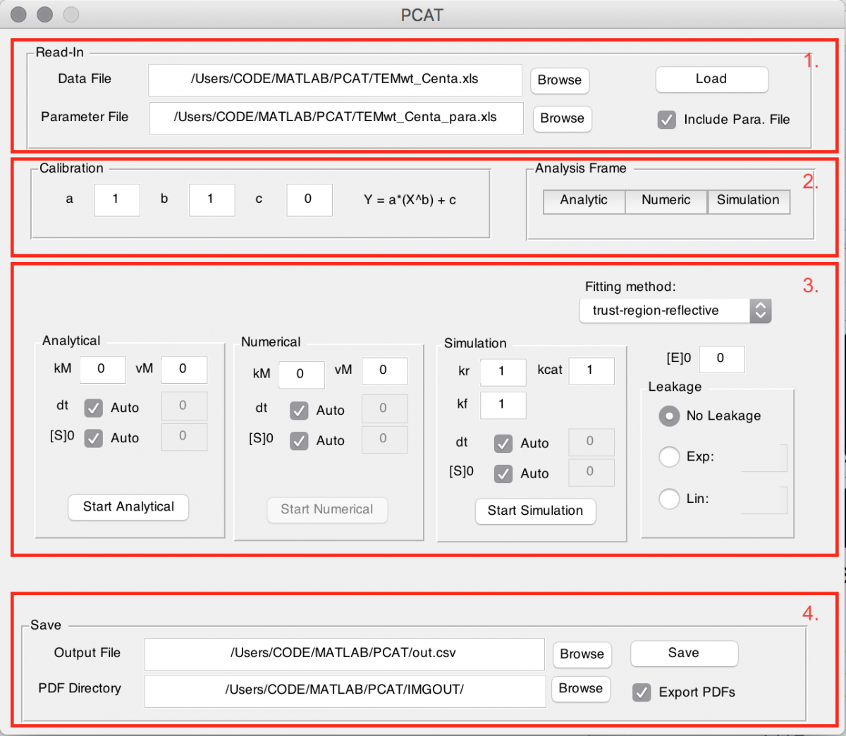
Once installation is complete the program can be called by the command PCAT in the Matlab command window. Optionally one can right click on the PCAT.m file in the current folder tab and select run. A graphical user interface (GUI) opens up which guides the analysis procedure (see figure).
The top part (1.) provides the possibility to read in a data file and a parameter file (which is optional, see input details).
You will find attached an “example data file” and an “example para file” that you can use for training. After selection of their location, either by directly inserting it, or by using the Browse button press the Load button.
The second part (2.) gives the option to specify calibration parameters for the data loaded and choose analysis frames for the three models. The calibration has a linear coefficient a, a power coefficient b and an offset coefficient c. Each can be specified either in the box for all datasets or individually in the parameter file. The calibration comes to relate the product signal to its real concentration. The analysis frame has to be set before one can proceed to the analysis. Again, this can be set in the parameter file. By clicking on the corresponding button (Analytic, Numeric or Simulation) a window opens up showing the outline of the data. With two clicks the frame is chosen, whereas the first selects the start point and the second the end point. Please always press directly on the plot. The next dataset immediately opens up when the previous one is selected. To cancel close the figure. If the start and end point have already been provided in the parameter file they need to be confirmed, also by clicking the corresponding button.
Once the frame has been selected the Start … buttons become available in the next section (3.). For each model the starting parameters can be set in the corresponding fields above the start button. The option Auto for dt and [S]0 automatically sets the start point from the analysis frame and the maximum concentration of dataset as initial conditions respectively. With the drop down menu in the upper right corner one can choose the fitting method. It is advised to use trust-region reflective mode, if unsure what the differences are. Enzyme concentration is only required for the analysis with the simulation model. However, it enables saving of catalytic efficiency and kcat for the other two models when used. In the Leakage box either none, an exponential or linear decay can be selected with the given initial condition. This is important if the progress curve slopes down at later times.
Before proceeding to analysis by pressing the Start … buttons, one can optionally enable exporting of a .fig and .pdf file with a tick box in the lower right corner (4.) – it is important to provide a location, folder respectively for those. During analysis a window shows the current progress of residuals and the resulting figure for every dataset even if saving is disabled. It is advised not to use Matlab for other purposes during the analysis step.
Lastly one can save all results in one row-separated .csv file by pressing the button Save.
Input details
PCAT loads data from a column-separated .xls file. The first column has to depict time and each following column is loaded as a dataset (they all share the same timestamps). The top row in the data file acts as naming placeholder and can contain any string. The time column must have at least as many entries as the longest dataset. Datasets can vary in length, but have to start from the second row on. See TEMwt_Centa.xls within the current folder list in Matlab as an example data file.
Optionally a parameter file can be loaded. It is also column-separated where the first column now gives a list of possible parameters to specify. There are as many columns required as there are datasets. The top row here also acts as a placeholder for naming of the datasets. For each dataset the parameters can be tuned individually and if left blank the corresponding parameter from the GUI will be chosen. Please use TEMwt_Centa_para.xls as a template. The suffixes _A, _N and _S stand for analytical, numerical and simulation respectively.
